


Compton Camera
A Compton Camera is used for imaging of photons in the energy range of 500 keV and above and makes use of the energy and momentum conservation in the Compton scattering process.
Compton imaging has specific applications notably:
- Low energy gamma ray (1-30 MeV) detection in astrophysics, e.g., COMPTEL Telescope aboard Compton Gamma-Ray Observatory (GRO) [1] and Nuclear Compton Telescope (NCT) [2].
- Gamma ray detectors in radioactive substance visualization cameras which are used mainly after nuclear power plant accidents [3].
- Gamma Ray detectors for medical imaging.
Compton Camera for Medical Imaging:
Radiotherapy is a promising method to eliminate cancer tissues. For instance, in Proton Beam Therapy (PBT), the beam deposits most of its energy in the Bragg peak. The challenge is to deliver precise dose in the desirable location. Otherwise, the healthy tissue might be irradiated or incorrect dose may be applied. Protons ionize and excite the irradiated tissue. The de-excitation of atoms in the tissue is accompanied by emission of gamma rays. Detection of these photons gives us precise information regarding location and dose of the proton beam. This is where Compton cameras come into play. They detect gamma rays in this range and determine their source location and energy.
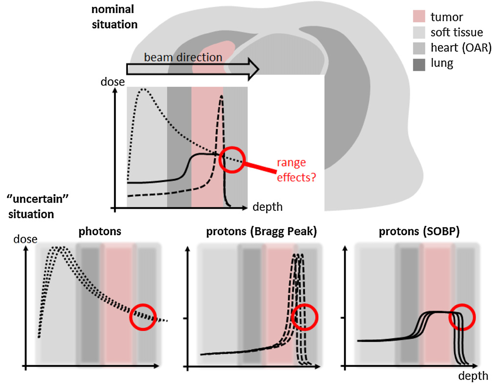
Comparison of photon treatment (dotted line) and mono-energetic proton beam including the Bragg peak (dashed line) and the spread-out Bragg peak consisting of several proton energies to cover the whole tumor volume [4]
Compton Camera: how does it work?
Compton camera is based on two physics phenomenon: Compton Scattering and Cherenkov Radiation
1. Compton Scattering (Scattering Light off Electrons)
The Compton scattering (along with black body radiation and photoelectric effect) was the nail in the coffin to the notion that classical physics alone can explain physics phenomenon in quantum scale. Although simple, the experiment cannot be explained by classical physics.
The Experiment:
If a photon with energies in the range of a few keV to 30 MeV (depending on the atomic number of the absorber material) hit an electron at rest, the photon will be scattered.
According to classical electromagnetism, the electron absorbs the photon, starts oscillating, and emits a photon with the same wavelength and intensity as the initial photon has. However, observations show that the emitted photon has greater wavelength and lower intensity.
Arthur Compton's explanation:
In 1923, Arthur Holly Compton at Washington University in St. Louis came up with a quantum explanation which earned him the 1927 Nobel Prize in Physics. He treated the photon as a discrete particle, not a wave. He further assumed that the photon collides with a single electron elastically and solved the mathematical equation for conservation of energy and momentum.
|
$\huge\lambda_{\gamma_{2}}-\lambda _{\gamma_{1}}-\frac{h}{m_{e}c}\left (1-\cos{\theta} \right)$ |
(1) |
|
$\huge E_{\gamma_{2}}=\frac{1}{\frac{1}{E_{\gamma_{1}}}+\frac{\left ( 1-cos\theta \right )}{m_{e}c^{2}}}$ |
(2) |
λγ1: Wavelength of the incident photon (m)
λγ2: Wavelength of the emitted photon (m)
Eγ1: Energy of the incident photon (eV)
Eγ2: Energy of the emitted photon (eV)
h: Planck Constant (≅ 4.14×10⁻¹⁵ $\frac{eV}{Hz}$)
me: Electron rest mass ($\frac{eV}{c^{2}}$)
c: Speed of light (≅ 3×10⁸ $\frac{m}{s}$)
θ: Scattering angle
$\mathbf{\frac{h}{m_{e}c}}$: Compton wavelength of electron (≅ 2.43×10⁻¹²m)
2. Cherenkov Radiation (Breaking the Light Barrier!)
Light travels with the speed of light c in vacuum and with $\mathbf{\frac{c}{n}}$ in a material with refractive index n. When a charged particle is traveling through a dielectric (Electrically polarizable) material, it creates electric dipoles in its path by locally polarizing the dielectric material. If the speed of the charged particle is smaller than or equal to $\mathbf{\frac{c}{n}}$, the electric dipoles elastically disappear as the particle moves past them. However, if the charged particle’s speed is larger than $\mathbf{\frac{c}{n}}$, the medium’s response becomes slower than the charged particle’s speed, and dipoles are left in the wake of the particle. The energy contained in this disturbance is radiated as a shockwave known as Cherenkov Radiation. The shockwave Travels at speed of light in the Medium ($\mathbf{\frac{c}{n}}$). That is, the shockwave still travels slower than Phase velocity of the charged particle.
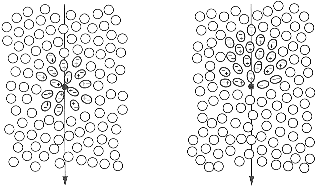
Polarization of a medium by a charged particle. Left: Charged particles have velocities smaller than $v>\frac{c}{n}$; dipoles elastically disappear as the particle passes. Right: Charged particles have velocities larger than $v>\frac{c}{n}$; Dipoles remain in the wake of the particle, causing Cherenkov Radiation. [5]
Cherenkov Light Emission Angle:
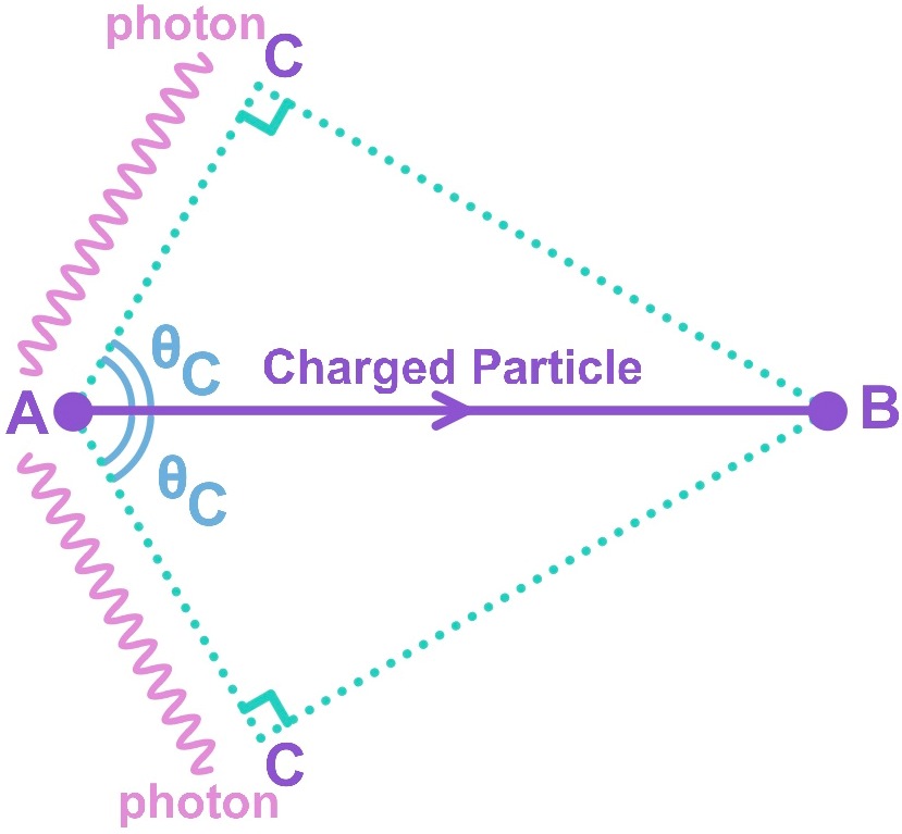
Cherenkov photons radiate in a cone shape with half angle θC
During the time t, the charged particle travels AB=vt in the medium, where v is the speed of the particle. If $\mathbf{v>\frac{c}{n}}$, the produced Cherenkov photons travel the distance $\mathbf{AC=t\times\frac{c}{n}}$ in the medium at an angle θC wrt the charged particle. Therefore, the Cherenkov photons are emitted in cone shape with half angle θC .
|
$\huge AB=vt=\beta ct$ |
(3) |
|
$\huge AC=\frac{c}{n}t$ |
(4) |
|
$\huge \cos \theta_{C}=\frac{AC}{AB}=\frac{1}{\beta n}$ |
(5) |
v: Speed of the charged particle in the medium ($\frac{m}{s}$)
β: Ratio of v over c (Dimensionless)
n: Refractive Index of the medium (Dimensionless)
θC: Cherenkov Emission Angle
Refractive index of a medium changes with wavelength of the charged particle due to dispersion relation. Hence, highly energetic particles have smaller Cherenkov angles.
Threshold Energy (E(Thresh.)):
From Equation (5), we can determine the minimum β at which Cherenkov emission occurs.
|
$\huge \beta_{Thresh.}=\frac{1}{n}$ |
(6) |
Equation (6) yields the minimum energy required to produce Cherenkov light. βThresh. depends only on refractive index. That is EThresh. changes only with n. Thus, knowledge of Threshold energy leads to knowledge of the rest mass of the charged particle, which is why Cherenkov Radiation is an ideal method for particle identification.
|
$\huge E_{Thresh.}=\gamma_{Thresh.}m_{0}c^{2}=\frac{1}{\sqrt{1-\beta_{Thresh.}^{2}}}m_{0}c^{2}$ |
(7) |
EThresh.: Threshold Energy (eV)
γThresh.: Threshold Lorentz Factor (Dimensionless)
Photon Yield of Cherenkov Radiation: $\mathbf{\frac{dN}{dx}}$
The number of produced Cherenkov photons with wavelengths between γ1 and γ2 per path length are defined as Cherenkov photon yield.
α: Fine Structure Constant ($\cong \frac{1}{137}$ - Dimensionless)
z: Particle's electric charge (e)
Current Research
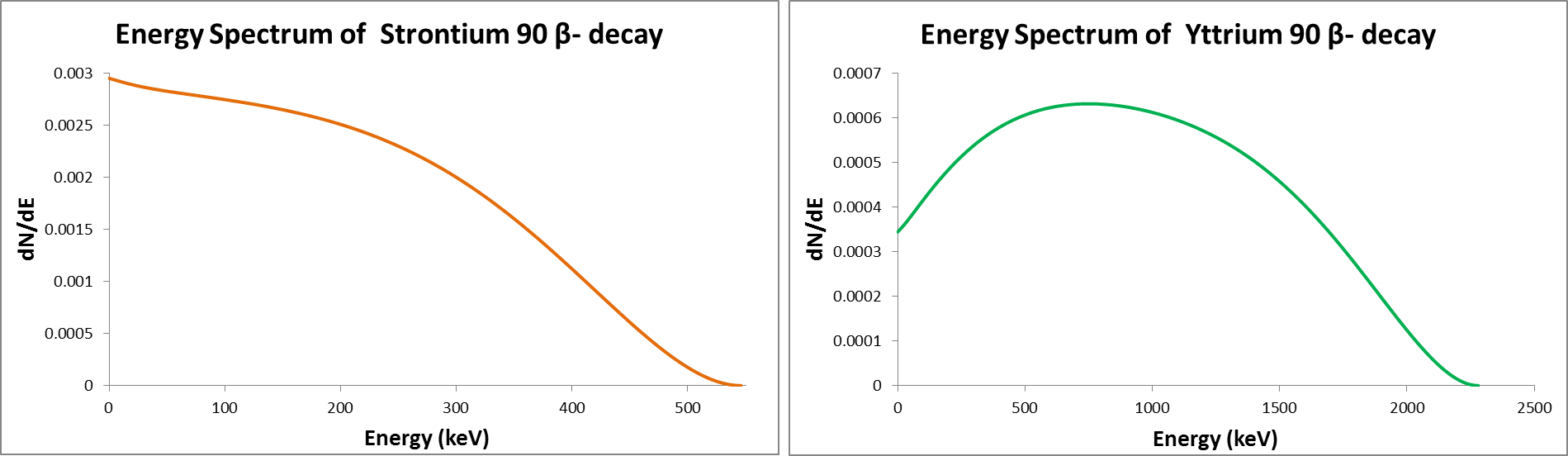
The (Compton) electrons are produced from beta minus decay of Strontium 90/Yttrium 90 with energies up to 2.28 MeV. Due to thre-body decay, beta particles have continuous energy range, peaking at small energies and reaching β end-point energy.
The electrons are detected via their Cherenkov radiation produced in an PMMA radiator. The Cherenkov photons are then detected with a SiPM.
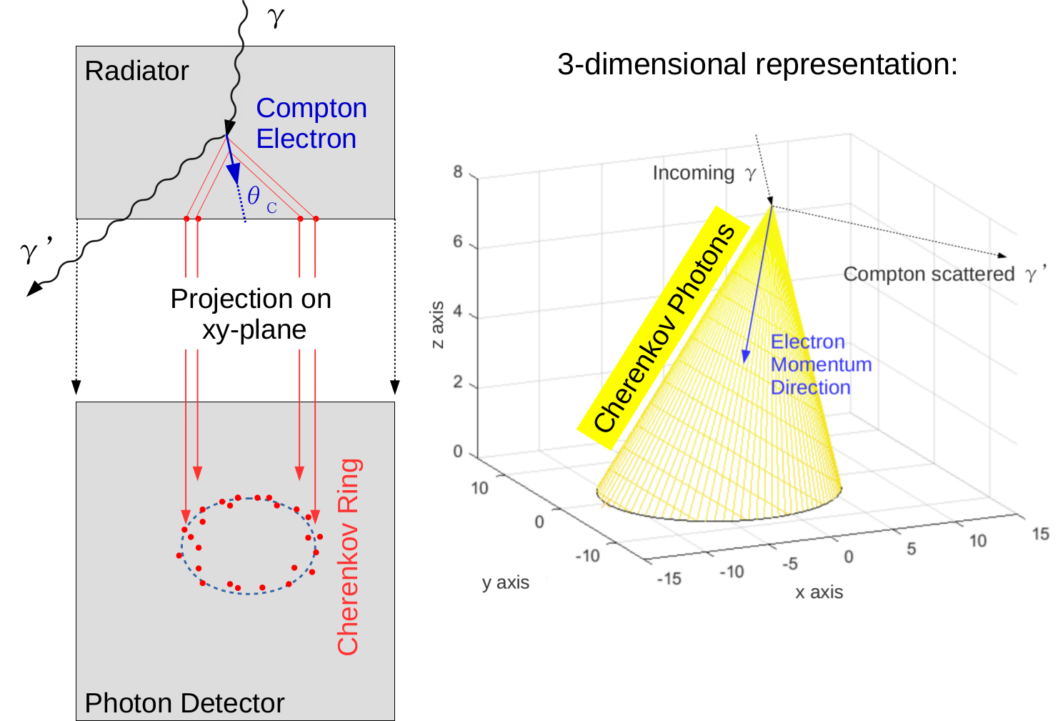
Compton electron detection using Cherenkov cone reconstruction [8]
In order to measure the amount of Cherenkov photons produced by an electron of a given energy a dedicated experiment has been contructed.
The electrons are directed through a vacuum channel within which an EM field from an electromagnet allows only a specific energy to reach a collimator at the end of the path due to Lorentz Force. The number of coil windings, permeability of the iron yoke, and dimension of the air gap of the electromagnet were determined from the magnetic field required to bend the electrons using Ampère's Circuital Law and three-dimensional Biot-Savart Law.
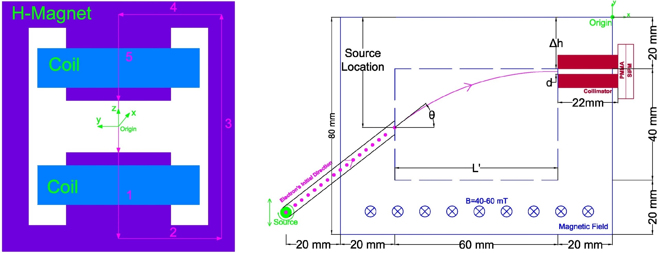
Left: Cross section of the magnet with Ampèrian Loop. Right: Schematics of the setup and the Magnet's air gap
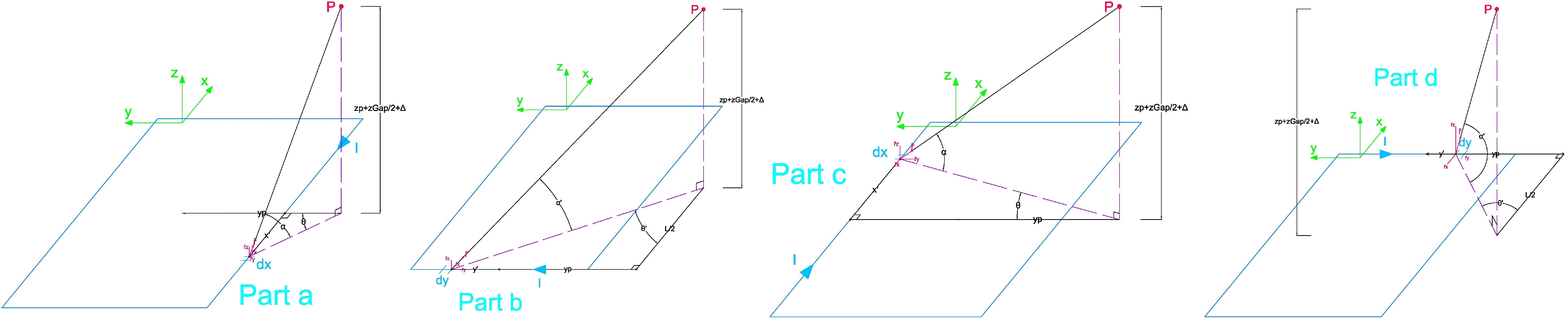
Implementation of 3-D Biot-Savart Law for section 3 of the Ampèrian Loop
To validate the theory, magnetic field is measured via Teslameters and homogeneous profile of the newly designed electromagnet is determined. The electron trajectory is then adjusted based on the measured magnetic field.
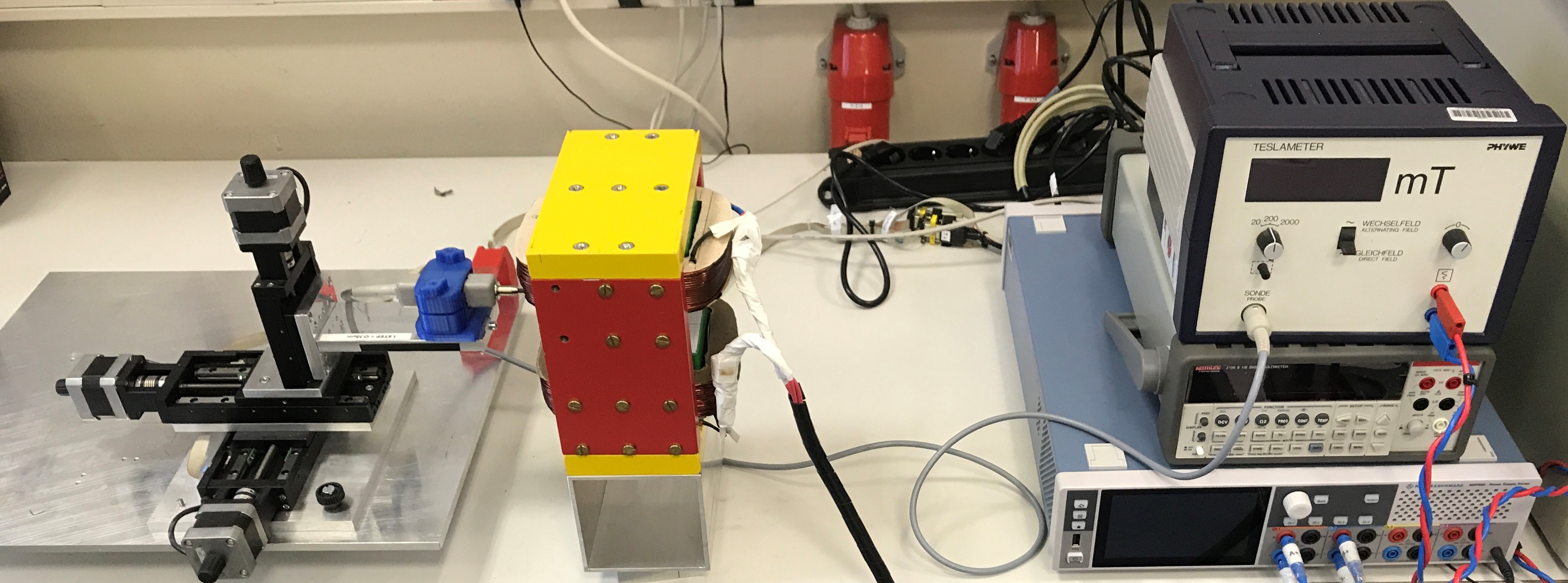
Magnetic field inside the magnet is measured using a tangential Hall probe, a teslameter, a power supply, a multimeter, and a high precision, 3-axis step motor
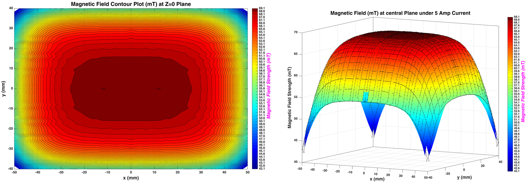
Left: Contour plot of the homogeneous section of the magnet. Right: 3D Magnetic profile of the magnet
After the collimator, the energy spread of the electrons is less than 6% around the nominal energy which can vary between 0.5 and 2.28 MeV.
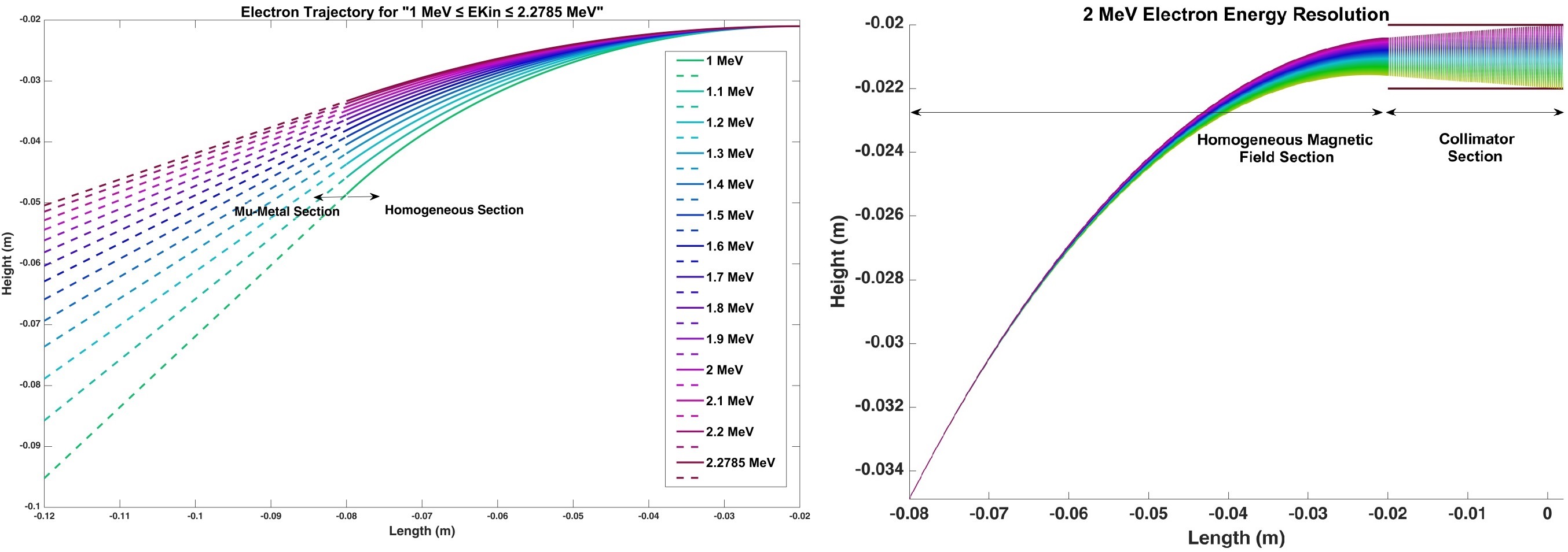
Left: Electron trajectory for high energies and 60 mT magnetic field strength. Energies are color coded, i.e., green represents lowest energy, and red represents highest energy. Right: Escaping energies when the main energy is 2 MeV and collimator size is 2x22mm. The horizontal lines represent the boundaries of the collimator.
The electrons subsequently reach a radiator material (PMMA) and produce Cherenkov photons, which are detected via a 8×8 Silicon-Photomultiplier array with 64 readout channels. For each electron, the Cherenkov photons are collected within a time-window of 100 ns. The spatial distribution of the Cherenkov photons and their total number are recorded and will be investigated as a function of electron energy, and the results will be compared with theoretical data.
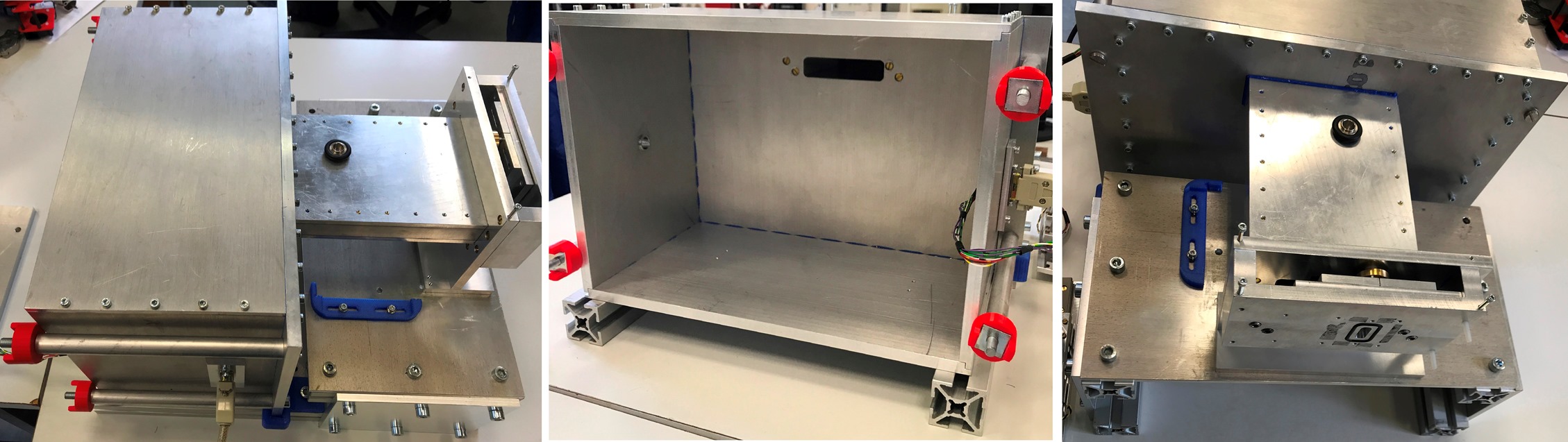
Left: Main vacuum chamber where the radioactive source, and positioning mechanism will be placed. Center: Top view of the setup. Right: Magnet's channel, collimator, and the entry through which the cherenkov photons reach the PMMA.
References:
- [1] Schoenfelder, V. et al., “Instrument Description and Performance of the Imaging Gamma-Ray Telescope COMPTEL aboard the Compton Gamma-Ray Observatory”, The Astrophysical Journal Supplement Series, vol. 86, p. 657, 1993. doi:10.1086/191794.
- [2] E. C. Bellm et al., "Overview of the Nuclear Compton Telescope", IEEE Transactions on Nuclear Science, vol. 56, no. 3, pp. 1250-1256, June 2009, doi: 10.1109/TNS.2009.2016091.
- [3] Tomono, D. et al. "First On-Site True Gamma-Ray Imaging-Spectroscopy of Contamination near Fukushima Plant", Sci Rep 7, 41972, 2017, doi: https://doi.org/10.1038/srep41972.
- [4] Knopf, A. & Lomax, A., "In vivo proton range verification: A review", Physics in medicine and biology, 58. R131-60, 2013, doi: 10.1088/0031-9155/58/15/R131.
- [5] Kolanoski, H. & Wermes, N., "Teilchendetektoren: Grundlagen und Anwendungen", Springer Spektrum, January 2016, doi: 10.1007/978-3-662-45350-6.
- [6] "Live Chart of Nuclides", International Atomic Energy Agency, Accessed December 2020, https://www-nds.iaea.org/.
- [7] Mougeot, X., "Reliability of usual assumptions in the calculation of β and ν spectra", Phys. Rev. C, vol. 91, 055504, May 2015, doi: 10.1103/PhysRevC.91.055504.
- [8] Bayerlein, R., "Coincident Detection of Cherenkov Photons for Medical Applications", PhD Thesis, University of Siegen, 2020.